Author: Dian Wang, Guiwen Guan
Introduction
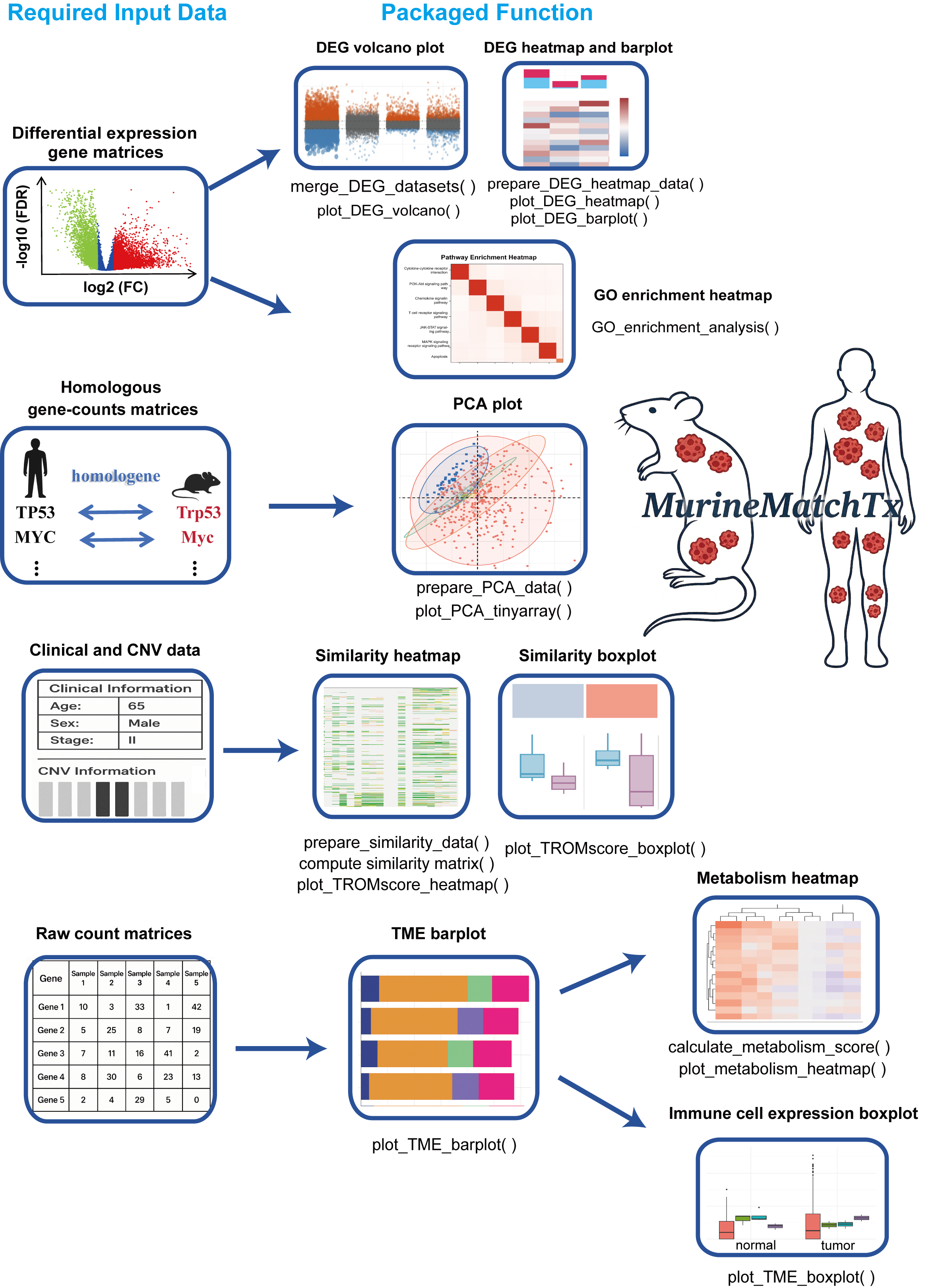
The Cross-Species Transcriptomic Similarity Analysis R package (MurineMatchTx) provides a comprehensive and user-friendly framework for evaluating transcriptional similarities between mouse cancer models and human cancer samples. Designed to streamline cross-species transcriptomic analysis, MurineMatchTx enables rapid, multidimensional exploration with minimal preprocessing—simply input standardized files following the provided guidelines.
The package integrates a wide array of functionalities, including differential expression gene integration and visualization, graphical display of PCA, transcriptional similarity scoring (TROM scores), immune infiltration profiling, and functional enrichment analysis (GO terms). Each function is highly customizable through flexible parameter settings, allowing researchers to tailor the analysis to specific experimental needs.
With MurineMatchTx, users can rigorously assess how closely animal models recapitulate the molecular features of human cancers, thereby facilitating translational research at the transcriptomic level.
Installation
You can install the package directly from GitHub:
# Install devtools if necessary
if (!require("devtools")) install.packages("devtools")

# Install the package
devtools::install_github("wangdian-PKU/MurineMatchTx")
General input files to be prepared in advance
We strongly suggest that all user - provided input files should be in the tsv format!!!
- Expression matrix: Differentially expressed gene matrix between the cancer group and the normal group in mouse models.
- Expression matrix: Differentially expressed gene matrix between human cancer group and the normal group (TCGA as examples).
- Clinical Data: human clinical metadata with patient IDs and different clinical conditions data.
- CNV Data: human CNV alterations of specified genes (e.g., TP53, PTEN).
Main Functions
1. Merge_DEG_datasets()— Merge differentially expressed data from human samples or mouse models
1.1 Purpose
The merge_DEG_datasets() function is designed to combine differential gene expression (DEG) results from TCGA (human) and multiple mouse cancer models into a unified, tidy data frame. This merged data can then be used to draw volcano plots of DEG downstream.
1.2 Input Data Format
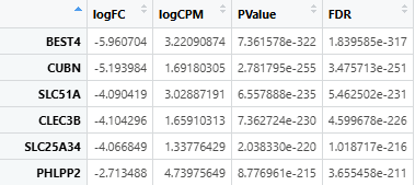
This function requires DEG result files from TCGA and mouse models in .tsv or .csv format. It can be derived from the DEG matrix generated by DESeq2 or edgeR. These files must:
- Be tab- or comma-separated.
- Include at least the following columns:
logFC: Log2 fold change of gene expression.FDR: False discovery rate (adjusted p-value).
- Row names should be gene symbols or gene identifiers.
Example .tsv or .csv format after being read:
1.3 Function Parameters
| Argument | Type | Default | Description |
|---|---|---|---|
| human_file_path | character | Required | File path to TCGA DEG file (.tsv or .csv). |
| mouse_files | named list | Required | Named list of file paths to mouse model DEG files. |
| logFC_value | numeric | 1 | Log2 fold change threshold to define “Up” or “Down” genes. |
| FDR_value | numeric | 0.05 | FDR threshold for statistical significance. |
1.4 Output
A merged data frame with the following columns:
| Column | Description |
|---|---|
| gene | Gene symbol (from row names) |
| logFC | Log2 fold change |
| FDR | Adjusted p-value |
| contrast | Dataset source (e.g., “TCGA”, “GSE172629”, “Our_Model”) |
| change | DEG status: “Up”, “Down” or “Stable” based on thresholds |
1.5 DEG Classification Logic
The function uses the following rule to classify gene expression change:
if (logFC > threshold & FDR < threshold) → "Up"
if (logFC < -threshold & FDR < threshold) → "Down"
otherwise → "Stable"
1.6 Run Example
# Define file paths
tcga_file <- "./data/TCGA_DEG.tsv"

mouse_files <- list(
  "Our_Model"   = "./data/Our_Model_DEG.csv",
  "GSE172629"   = "./data/GSE172629_DEG.tsv",
  "GSE208279"   = "./data/GSE208279_DEG.tsv"
)

# Merge datasets with default thresholds
merged_DEG <- merge_DEG_datasets(
  human_file_path = tcga_file,
  mouse_files = mouse_files
)

# Optional: custom thresholds
merged_DEG_custom <- merge_DEG_datasets(
  human_file_path = tcga_file,
  mouse_files = mouse_files,
  logFC_value = 1.5,
  FDR_value = 0.01
)

# View result
head(merged_DEG)
1.7 Downstream Use Cases
- As input for
plot_DEG_volcano()functions. - For cross-species DEG pattern comparison.
1.8 Notes
- The
genecolumn is automatically added from rownames of each DEG file. - If the input files contain missing or invalid values, the function will throw warnings or errors.
- File format must be
.tsvor.csv, other formats (e.g., Excel.xlsx) are not supported directly.
2. plot_DEG_volcano()— Volcano Plot for Differential Expression Analysis
2.1 Purpose
The plot_DEG_volcano() function generates a volcano plot for visualizing differential expression results, highlighting significantly upregulated, downregulated, and stable genes, and also used to illustrate transcriptomic differences between experimental groups.
2.2 Input Data Format
This function requires a data frame (output from merge_DEG_datasets()) with the following mandatory columns:
| Column | Type | Description |
|---|---|---|
| gene | character | Gene name |
| logFC | numeric | Log2 fold change of gene expression |
| FDR | numeric | False discovery rate(adjusted p-value) |
| contrast | character/factor | Sample group identifier(e.g. TCGA, GSE…) |
| change | character | Gene status: “Up”, “Down”, or “Stable” |
Tip: Use merge_DEG_datasets() to generate this standardized input data frame.
2.3 Function Parameters
| Parameter | Type | Default | Description |
|---|---|---|---|
| deg_data | data.frame | Required | DEG results including required columns |
| title | character | “Volcano Plot of DEG Analysis” | Plot title |
| xlab | character | “Group” | X-axis label |
| ylab | character | “Log2 Fold Change” | Y-axis label |
| colors | named list | list(Up = "#e6550d", Down = "#3182bd", Stable = "#636363") |
Colors for DEG categories |
| point_size | numeric | 2 | Dot size |
| alpha_range | numeric | c(0.3, 1) | Transparency range based on FDR |
| x_angle | numeric | 45 | X-axis label angle |
| legend_position | character | “right” | Legend position: “right”, “top”, “bottom”, “left”, “none” |
| width | numeric | 10 | Plot width in inches |
| height | numeric | 6 | Plot height in inches |
| output_path | character | "./DEG/" |
Folder path to save output PDF |
2.4 Output
- Visual Output: A ggplot object showing genes grouped by contrast, with log2 fold change on the Y-axis and group on the X-axis. The color and size of each point reflects gene regulation status and significance.
- File Output:
A PDF file named
volcano_plot.pdfwill be saved to the specifiedoutput_path.
2.5 Run Example
# Prepare merged DEG data (e.g. from TCGA and mouse models)
merged_data <- merge_DEG_datasets(
  human_file_path = "./data/TCGA_DEG.tsv",
  mouse_files = list(
    "GSE172629" = "./data/GSE172629_DEG.tsv",
    "GSE208279" = "./data/GSE208279_DEG.tsv"
  )
)

# Generate volcano plot with default settings
p <- plot_DEG_volcano(deg_data = merged_data)

# Display the plot
p

# Further customization using ggplot2
p + ggplot2::theme_minimal()
2.6 Notes
- Dot color is determined by the
changecolumn (e.g., “Up”, “Down”, “Stable”). - Transparency and dot size are proportional to
-log10(FDR).
3. prepare_DEG_heatmap_data()— Process DEGs data for Heatmap Visualization
3.1 Purpose
The prepare_DEG_heatmap_data() function processes differential expression gene (DEG) results from TCGA and multiple mouse models to prepare a standardized dataset suitable for heatmap visualization. It performs significance filtering, homologous gene conversion, and logFC simplification, returning cleaned and comparable list of matrices for downstream visualization.
3.2 Input Data Format
See the file format requirements in the merge_DEG_datasets() documentation.
Each DEG file (both TCGA and mouse) must contain at least the following columns:
logFC– log2 fold changeFDR– false discovery rate (adjusted p-value)
Files must be in .tsv format and have gene identifiers as row names.
3.3 Function Parameters
| Argument | Type | Default | Description |
|---|---|---|---|
| tcga_file | character | Required | Path to the TCGA DEG .tsv file. |
| mouse_files | list | Required | A named list of file paths to mouse DEG .tsv files. Names will be used as column prefixes. |
| inTax | numeric | 9606 | Input species taxonomy ID (default: 9606 = human). |
| outTax | numeric | 10090 | Output species taxonomy ID (default: 10090 = mouse). |
3.4 What the Function Does
-
Load and Filter TCGA Data:
-
Reads the TCGA DEG file.
-
Selects genes with
|logFC| ≥ 1andFDR < 0.05.
-
-
Convert Human Genes to Mouse Homologs:
-
Uses
homologene::homologene()to map human genes to mouse homologs. -
Only genes with successful mappings are retained.
-
-
Count Up/Downregulated Genes:
- Separates positive (
logFC > 0) and negative (logFC < 0) genes.
- Separates positive (
-
Format TCGA logFC Values:
-
Upregulated: logFC set to
1 -
Downregulated: logFC set to
-1 -
Others: set to
NA
-
-
Process Mouse Model Files:
- For each file:
- Subsets rows to match TCGA homologs.
- Retains only
logFCandFDRcolumns.
- For each file:
3.5 Output
Returns a named list with the following components:
| Name | Type | Description |
|---|---|---|
| processed_tcga | data.frame | Filtered and formatted TCGA DEG matrix |
| processed_mouse | list | List of processed mouse model DEG matrices, each with standardized logFC values |
| tcga_gene_list | character vector | Final set of homologous genes retained in analysis |
3.6 Run Example
# Define file paths
tcga_path <- "./data/TCGA_DEG.tsv"
mouse_files <- list(
  "Our_Model" = "./data/Our_Model_DEG.tsv",
  "GSE172629" = "./data/GSE172629_DEG.tsv"
)

# Run preprocessing
processed_data <- prepare_DEG_heatmap_data(tcga_path, mouse_files)

# View output
head(processed_data$processed_tcga)
head(processed_data$processed_mouse$Our_Model)
3.7 Note
- The returned output is ready for use in the
plot_DEG_heatmap()functions. - The logFC simplification logic ensures compatibility across datasets and makes interpretation of heatmaps more intuitive.
4. plot_DEG_heatmap()— Visualize Differential Expression Patterns in a Heatmap
4.1 Purpose
The plot_DEG_heatmap() function generates a binary expression heatmap (values of 1, -1, or NA) across multiple mouse models based on TCGA-derived significant genes. It is intended to highlight genes with high or low expression in TCGA tumors and examine their cross-species expression trends in mouse models.
This function is typically used after preparing input data with prepare_DEG_heatmap_data().
4.2 Input Data Format
- This function expects the
deg_datato be the output fromprepare_DEG_heatmap_data().
4.3 Function Parameters
| Argument | Type | Default | Description |
|---|---|---|---|
| deg_data | list | Required | Output from prepare_DEG_heatmap_data(), containing filtered and formatted TCGA/mouse DEG data. |
| mouse_files | list | Required | The original named list of mouse model DEG paths used as input to prepare_DEG_heatmap_data(). |
| col_names | character | NULL | Optional custom column names for heatmap (default uses names from mouse_files). |
| cluster_rows | logical | FALSE | Whether to cluster the rows (genes). |
| cluster_cols | logical | FALSE | Whether to cluster the columns (models). |
| color_palette | named vector | c("1" = "#ff7676", "-1" = "#66d4ff", "NA" = "white") |
Color mapping for high/low/NA gene values. |
| width | numeric | 7.9 | Width of the output PDF plot. |
| height | numeric | 5.95 | Height of the output PDF plot. |
| output_path | character | "./DEG/" |
Path to save the output heatmap PDF file. |
4.4 What the Function Does
- Validates Input:
- Ensures that
deg_datacontains the expected structure.
- Ensures that
- Combines Mouse Model Data:
- Extracts
logFCinformation from each mouse model dataset. - Combines them into a single binary matrix (
merge_edger) using the TCGA gene set.
- Extracts
- Assigns Row/Column Labels:
- Gene symbols are used as rownames.
- Column names are either taken from
mouse_filesor user-defined viacol_names.
- Plots Binary Expression Matrix:
1→ gene highly expressed in TCGA tumor samples.-1→ gene lowly expressed in TCGA tumor samples.NA→ not significant or not conserved.- Color-coded as red (up), blue (down), and white (NA).
- Drawn using
ComplexHeatmap::Heatmap()and saved to PDF.
- Returns Processed Matrix:
- Output matrix can be reused in downstream plots (e.g.,
plot_DEG_barplot()).
- Output matrix can be reused in downstream plots (e.g.,
4.5 Output
- A PDF heatmap saved to the provided
output_path. - The function also returns the merged matrix (
merge_edger) used forplot_DEG_barplot().
4.6 Color Legend
| Value | Meaning | Default Color |
|---|---|---|
| 1 | Highly expressed in tumor | #ff7676 (red) |
| -1 | Lowly expressed in tumor | #66d4ff (blue) |
| NA | Non-significant / Not matched | white |
Legend labels:
"Highly expression in tumor"=1"Low expression in tumor"=-1
4.7 Run Example
# Process DEG data
processed_data <- prepare_DEG_heatmap_data(tcga_file, mouse_files)

# Generate heatmap
merge_edger <- plot_DEG_heatmap(
  deg_data = processed_data,
  mouse_files = mouse_files
)
4.8 Notes
- This function is tightly coupled with
prepare_DEG_heatmap_data()— don’t use it with arbitrary input. - You can reuse
merge_edgerfor barplot visualization viaplot_DEG_barplot().
5. plot_DEG_barplot()— Barplot of DEG Counts in Mouse Models
5.1 Purpose
The plot_DEG_barplot() function generates a stacked barplot to compare the number of upregulated and downregulated genes in each mouse model, based on TCGA-derived gene categories. It uses the DEG matrix generated by the plot_DEG_heatmap() function.
5.2 Input Data Format
-
The function requires a matrix (
merge_edger) as input, which must be the output ofplot_DEG_heatmap()and contain:-
Rows: Filtered genes shared with TCGA.
-
Columns: Mouse models.
-
Values:
1for genes upregulated in TCGA tumors.-1for downregulated genes.NAfor genes not meeting the threshold or unmatched.
-
5.3 Function Parameters
| Argument | Type | Default | Description |
|---|---|---|---|
| heatmap_data | matrix | Required | The DEG matrix from plot_DEG_heatmap(), indicating expression patterns per model. |
| colors | list | list(up = "#ff7676", down = "#66d4ff") |
Colors used for up/down-regulated genes. |
| width | numeric | 8 | Width of the saved PDF plot. |
| height | numeric | 4 | Height of the saved PDF plot. |
| output_path | character | "./DEG/" |
Directory to save the output barplot. |
5.4 What the Function Does
- Validates Input:
- Checks that the input is a matrix with numeric values (
1,-1,NA).
- Checks that the input is a matrix with numeric values (
- Transforms Matrix to Long Format:
- Converts the wide-format DEG matrix into long format for
ggplot2.
- Converts the wide-format DEG matrix into long format for
- Assigns Group Labels:
- Converts values to
"up"(for1) or"down"(for-1) gene categories. - NA values are excluded.
- Converts values to
- Generates Barplot:
- X-axis: Mouse model names (
contrast). - Y-axis: Count of up/down genes per model.
- Colors: Customizable (default: red for up, blue for down).
- Uses
ggplot2::geom_bar()to generate a clean stacked barplot.
- X-axis: Mouse model names (
- Saves Output:
- Barplot is saved as
"barplot.pdf"inside the specifiedoutput_path.
- Barplot is saved as
5.5 Output
| Output | Type | Description |
|---|---|---|
| Barplot (PDF) | file | A visual file saved to disk. |
| Plot Object | ggplot | The plot is returned as a ggplot object for further customization. |
5.6 Color Legend
| Group | Value in Matrix | Color |
|---|---|---|
| Upregulated | 1 | "#ff7676" (red) |
| Downregulated | -1 | "#66d4ff" (blue) |
You can change colors via the colors argument, for example:
colors = list(up = "red", down = "blue")
5.7 Run Example
# Generate barplot from merge_edger matrix
barplot <- plot_DEG_barplot(
  heatmap_data = merge_edger,
  colors = list(up = "#ff7676", down = "#66d4ff")
)

# Display in RStudio
print(barplot)
5.8 Notes
- This function is intended to be used after
plot_DEG_heatmap(). - Genes not matched or not significantly regulated (
NA) are automatically excluded. - The returned
ggplotobject allows additional customization using the fullggplot2ecosystem.
6. prepare_PCA_data()- prepare data for PCA plotting
6.1 Purpose
The prepare_PCA_data() function merges TCGA and mouse model expression data, assigns group and batch labels, and optionally performs batch correction. This prepares the data for PCA analysis and plotting of transcriptional similarity in downstream function plot_PCA_tinyarray().
6.2 Input Data Format
Before you wanna using this fuction, you should first obtain the homologous gene-counts matrix files for TCGA and each mouse model, which could be obtained via the homologene package. The specific code and the expected data is as follows:
# For TCGA
count <- read.table("./TCGA.rawcounts")
library(homologene)
homolo_gene <- homologene(rownames(count), inTax = 9606, outTax = 10090)[,c(1:2)]
count <- count[rownames(count) %in% homolo_gene[, 1], ]
rownames(count) <- toupper(rownames(count))
count <- rownames_to_column(count,var = "X") # The var parameter must set as "X"


# For mouse model
count <- read.table("./GSE.rawcounts")
library(homologene)
homolo_gene <- homologene(rownames(count), inTax = 10090, outTax = 9606)[,c(1:2)]
count <- count[rownames(count) %in% homolo_gene[, 1], ]
rownames(count) <- toupper(rownames(count))
count <- rownames_to_column(count,var = "X") # The var parameter must set as "X"
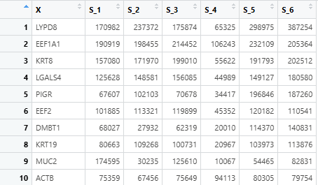
The input expression files (for both TCGA and mouse models) must:
- Be in
.tsvor.csvformat. - Contain homologene symbols as the first column (colnames =
X).
6.3 Function Parameters
| Parameter | Type | Default | Description |
|---|---|---|---|
| tcga_file | Character | Required | File path to TCGA expression matrix (.csv or .tsv). |
| mouse_files | Named list | Required | Named list of expression matrix paths for mouse models. |
| sample_counts | Named list | Required | Sample size info per dataset: normal and tumor count. |
| batch_correction | Logical | TRUE | Whether to apply ComBat batch correction. Default: TRUE. |
6.4 What the Function Does
- Reads TCGA and mouse model expression files.
- Merges all datasets using gene symbols.
- Generates:
group_all: sample group labels likeTCGA_normal,GSExxx_tumor.batch: batch labels for each dataset.
- Applies batch correction using
sva::ComBat()if enabled.
6.5 Output
Returns a list containing:
| Output | Type | Description |
|---|---|---|
| merged_data | matrix | Merged raw expression matrix (genes × samples). |
| group_all | character | Sample group labels for PCA visualization. |
| batch | character | Batch information (dataset origin per sample). |
| corrected_data | matrix | Batch-corrected matrix (if batch_correction = TRUE). Otherwise NULL. |
6.6 Run Example
mouse_files <- list(
  "GSE172629" = "./data/GSE172629.homo.tsv",
  "GSExxxxxx" = "./data/GSExxxxxx.homo.csv"
)

sample_counts <- list(
  "TCGA" = c(normal = 50, tumor = 374),
  "GSE172629" = c(normal = 3, tumor = 3)
)

pca_data <- prepare_PCA_data(
  tcga_file = "./data/TCGA.tsv",
  mouse_files = mouse_files,
  sample_counts = sample_counts,
  batch_correction = TRUE
)
6.7 Notes
- File formats are automatically detected (
.tsvor.csv). - All gene sets across datasets must be aligned (same gene order after merge).
- If sample counts do not match actual column numbers, an error is thrown.
- The output
corrected_datais ready for PCA, clustering, or heatmap visualization.
7. plot_PCA_tinyarray()- PCA visualization
7.1 Purpose
The plot_PCA_tinyarray() function performs principal component analysis (PCA) and visualizes the result using the tinyarray::draw_pca() function. It supports both raw and batch-corrected expression matrices and highlights sample grouping with customizable colors.
7.2 Input Data Format
The function expects a list object returned from prepare_PCA_data(), which includes:
- A merged expression matrix (
merged_data) - Batch labels (
batch) - Sample group labels (
group_all)
- An optional batch-corrected matrix (
corrected_data)
7.3 Function Parameters
| Parameter | Type | Default | Description |
|---|---|---|---|
| pca_data | List | Required | Output from prepare_PCA_data(), must contain merged and optionally corrected matrices. |
| batch_correction | Logical | TRUE | Whether to use batch-corrected matrix for PCA plotting. |
| colors | Character vector | NULL | Custom color palette for groups. If NULL, default color palette is used. |
7.4 What the Function Does
- Selects batch-corrected or raw merged data depending on the
batch_correctionflag. - Converts sample group vector into a factor.
- Automatically assigns or validates colors for each sample group.
- Performs PCA using
tinyarray::draw_pca(), generating a 2D PCA plot with group labels and coloring.
7.5 Output
This function does not return an object, but directly draws the PCA plot to the active graphic device (RStudio Plots pane, PDF, etc.) for personalized adjustment.
7.6 Run Example
# Assume you have run `prepare_PCA_data()` and stored the result in `pca_data`

plot_PCA_tinyarray(
  pca_data = pca_data,
  batch_correction = TRUE  # Use ComBat-corrected data
)

# Customize colors manually (optional)
custom_colors <- c("#1b9e77", "#d95f02", "#7570b3")
plot_PCA_tinyarray(
  pca_data = pca_data,
  batch_correction = FALSE,
  colors = custom_colors
)
7.7 Notes
- If
batch_correction = TRUE, but nocorrected_dataexists in the input list, the function falls back to using the original merged data. - Ensure that
group_allmatches the number and order of samples in the expression matrix. - Default colors support up to 15 groups. Beyond that, manually define a longer
colorsvector.
8. prepare_similarity_data()- combine CNV and clinical file for similarity analysis
8.1 Purpose
This function prepares TCGA patient-level clinical and CNV (copy number variation) information for use in cross-species similarity analysis with mouse models. It extracts user-defined clinical risk factors(condition) and CNV data for selected genes and merges them into a clean, analysis-ready data frame.
8.2 Input Data Format
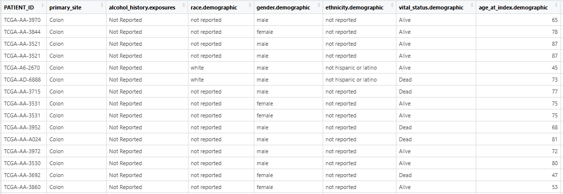
- The input clinical_file must be separated by tabs and contain the column named “PATIENT_ID”. And the character value in “PATIENT ID” should be unique!!! The table read using
read.table(clinic_file_path, header = TRUE, sep = "\t", stringsAsFactors = FALSE)is presented in the figure.
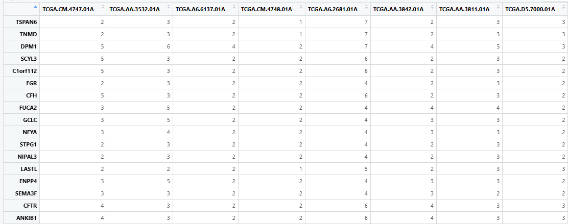
- The input cnv_file should be a tab-separated dataframe with rows representing gene symbols and columns representing TCGA PATIENT_IDs. The table read using
read.table (cnv_file_path, header=TRUE, sep="\ t", stringsAsFactors=False)is presented in the figure.
8.3 Function Parameters
| Parameter | Type | Default | Description |
|---|---|---|---|
| clinic_file | character | Required | Path to the TCGA clinical file (e.g., data_bcr_clinical_data_patient.tsv). |
| cnv_file | character | Required | Path to the TCGA CNV data file (e.g., CNA.tsv). |
| clinical_vars | character | Required | A character vector of user-defined clinical risk factors to extract. |
| cnv_genes | character | Required | A character vector of gene names (e.g., TP53, PTEN) to extract from CNV. |
| risk_factor_column | character | Required | The column name in the clinical file that contains different patient conditions. |
8.4 What the Function Does
- Reads the clinical and CNV data from TCGA
.tsvfiles. - Extracts only the
PATIENT_IDcolumn and the user-specified clinical variables (via pattern matching). - Selects only CNV data rows corresponding to the user-specified
cnv_genes. - Merges CNV and clinical variables into a unified matrix using
PATIENT_IDas the key. - Encodes CNV values as ordered factors with levels
-2,-1,0,1.
8.5 Output
A data frame containing:
- PATIENT_ID: Unique patient ID (standardized with
.instead of-) - One column per
clinical_vars, with matched status (or NA if not present) - One column per
cnv_genes, representing CNV status (-2,-1,0, or1) as factors
This merged output is used as input in downstream similarity scoring functions (e.g., compute_similarity_matrix() → plot_TROMscore_heatmap()).
8.6 Run Example
merge_clinic_CNV <- prepare_similarity_data(
  clinic_file = "data_bcr_clinical_data_patient.tsv",
  cnv_file = "CNA.tsv",
  clinical_vars = c("Hepatitis B", "Non-Alcoholic"),
  cnv_genes = c("TP53", "PTEN"),
  risk_factor_column = "HISTORY_HEPATO_CARCINOMA_RISK_FACTORS"
)
8.7 Notes
- The
clinical_varswill be matched by partial string search (case-insensitive) in the column defined byrisk_factor_column. - The resulting data frame is critical for annotating heatmaps and stratifying patients based on underlying genetic and clinical profiles.
9. compute_similarity_matrix()- Calculate similarity score
9.1 Purpose
The compute_similarity_matrix() function calculates a transcriptional similarity matrix between TCGA samples and mouse models, using the ws.trom() algorithm from the TROM package. It filters the similarity matrix to retain only biologically meaningful comparisons (tumor-tumor and normal-normal) and merges the filtered matrix with TCGA clinical and CNV data for downstream analysis.
9.2 Input Data Format
The input expression_matrix should be the batch-corrected expression matrix (typically the output from prepare_PCA_data()), where:
- Rows represent genes.
- Columns represent TCGA and mouse model samples.
- Row names are gene symbols.
The input merge_clinic_CNV is the processed clinical + CNV data result from prepare_similarity_data()
9.3 Function Parameters
| Parameter | Type | Default | Description |
|---|---|---|---|
| expression_matrix | matrix | Required | Batch-corrected expression matrix (genes × samples). |
| group_all | charactor | Required | Vector of sample group labels for TCGA and mouse models. |
| tcga_sample_size | numeric | Required | Total number of TCGA samples. |
| tcga_normal_count | numeric | Required | Number of normal samples in TCGA cohort. |
| merge_clinic_CNV | data frame | Required | Data frame containing TCGA clinical and CNV data (from prepare_similarity_data()). |
| cnv_genes | charactor | Required | Character vector of CNV genes to include in the output. |
| clinical_vars | charactor | Required | Character vector of clinical variables to include in the output. |
9.4 What the Function Does
- Calculates transcriptional similarity matrix using
TROM::ws.trom()between TCGA and mouse models. - Filters out irrelevant comparisons:
- Removes tumor-normal and normal-tumor comparisons.
- Retains only tumor-tumor and normal-normal similarities.
- Appends clinical annotations and CNV data to the filtered matrix.
- Sorts the final matrix by tissue type and clinical/CNV variables.
9.5 Output
The function returns a named list with two components:
similarity_matrix: The full similarity matrix (unfiltered), as computed byws.trom().dm_trom_del_backgroud_clinic: The filtered similarity matrix (excluding background noise), merged with clinical and CNV data for use inplot_TROMscore_heatmap()andplot_TROMscore_boxplot().
9.6 Run Example
similarity_results <- compute_similarity_matrix(
  expression_matrix = pca_data$corrected_data,
  group_all = pca_data$group_all,
  tcga_sample_size = 424,
  tcga_normal_count = 50,
  merge_clinic_CNV = merge_clinic_CNV,
  cnv_genes = c("TP53", "PTEN"),
  clinical_vars = c("Hepatitis B", "Non-Alcoholic")
)
9.7 Notes
ws.trom()performs cross-species comparison based on gene expression similarity and returns a matrix of TROM scores.- The filtering step ensures that only biologically comparable samples (tumor vs. tumor, normal vs. normal) are retained.
- The function requires accurate
group_alllabeling, where TCGA samples are listed first. - The
PATIENT_IDis inferred from the first 12 characters of TCGA sample IDs.
10. plot_TROMscore_heatmap()- TROM similarity score heatmap visualization
10.1 Purpose
The plot_TROMscore_heatmap() function generates a heatmap visualization of transcriptional similarity scores (TROM scores) between TCGA samples and mouse cancer models. It provides a high-level overview of how closely mouse models resemble different human tumor subtypes at the transcriptomic level. It also integrates CNV and clinical information in TCGA samples.
10.2 Input Data Format
dm_trom_del_backgroud_clinic: The data frame fromcompute_similarity_matrix(), containing filtered similarity scores merged with clinical and CNV data.trom_matrix: The data frame fromcompute_similarity_matrix(), containing the raw TROM similarity matrix before background filtering.- Sample groupings and counts must match those used in earlier PCA and similarity computations (e.g., from
prepare_PCA_data()andcompute_similarity_matrix()).
10.3 Function Parameters
| Parameter | Type | Default | Description |
|---|---|---|---|
| dm_trom_del_backgroud_clinic | data frame | Required | Data frame with filtered similarity scores and clinical annotations. |
| trom_matrix | matrix | Required | Raw similarity matrix from ws.trom() (before filtering). |
| tcga_sample_size | numeric | Required | Total number of TCGA samples. |
| tcga_normal_count | numeric | Required | Number of normal samples in TCGA. |
| model_group_count | numeric | Required | Total number of mouse model samples. |
| condition | named list | Required | Named list defining sample counts per mouse model condition. |
| clinical_vars | character | Required | Vector of clinical variables to annotate (e.g., “Hepatitis B”). |
| cnv_genes | character | Required | Vector of CNV genes used for annotations (e.g., “TP53”, “PTEN”). |
| group_all | character | Required | Vector with group labels from prepare_PCA_data(). |
| width | numeric | 11.84 | Width of the output PDF heatmap. |
| height | numeric | 7.11 | Height of the output PDF heatmap. |
| output_path | character | "./similarity/TROM_heatmap.pdf" |
Path to save the heatmap figure. |
| cluster_rows | logical | FALSE | Whether to cluster rows in the heatmap. |
| cluster_cols | logical | FALSE | Whether to cluster columns in the heatmap. |
10.4 What the Function Does
- Extracts TROM scores for TCGA and mouse model samples.
- Computes average TROM scores for each mouse model group (tumor/normal).
- Formats the similarity matrix into a structure suitable for
ComplexHeatmap. - Adds two layers of annotations:
- Column annotations: whether each mouse model sample is tumor or normal.
- Row annotations: TCGA clinical and CNV information.
- Draws and saves the heatmap using the
ComplexHeatmappackage.
10.5 Output
The function returns a list with two elements:
heatmap_obj: The drawn heatmap object (fromComplexHeatmap::draw()).merge_long: A long-format data frame containing:x: Mouse model sample label.y: Mean similarity score.group: Tumor or normal.condition: Experimental model condition.score: Rounded average TROM score.
This merge_long object is used directly as input for plot_TROMscore_boxplot().
10.6 Run Example
heatmap_results <- plot_TROMscore_heatmap(
  dm_trom_del_backgroud_clinic = similarity_results$dm_trom_del_backgroud_clinic,
  trom_matrix = similarity_results$similarity_matrix,
  tcga_sample_size = 424,
  tcga_normal_count = 50,
  model_group_count = 52,
  condition = list("HBV pten p53 ko" = 5, "DEN Cl4" = 16),
  clinical_vars = c("Hepatitis B", "Non-Alcoholic"),
  cnv_genes = c("TP53", "PTEN"),
  group_all = pca_data$group_all,
  output_path = "./similarity/TROM_heatmap.pdf"
)
10.7 Notes
- This heatmap emphasizes tumor-to-tumor and normal-to-normal transcriptional similarity across species.
- Colors are mapped from low (white) to high (deep red) TROM scores using
circlize::colorRamp2(). - Clinical annotations are reversed (
rev()) to align correctly with TCGA row order in the matrix. - The
merge_longresult can be reused for barplots or boxplots of similarity scores. - The function automatically creates directories if
output_pathdoes not exist.
11. plot_TROMscore_boxplot()- TROM similarity score boxplot visualization
11.1 Purpose
The plot_TROMscore_boxplot() function generates two types of plots to visualize transcriptional similarity scores (TROM scores):
- A boxplot that compares TROM scores between tumor and normal groups across mouse models.
- A tileplot that displays the average TROM score for each mouse model.
These visualizations help assess which mouse models best resemble specific TCGA tumor profiles.
11.2 Input Data Format
- The input
merge_longshould be the output fromplot_TROMscore_heatmap(), a data frame in long format containing:x: sample labelsy: TROM scoregroup: “tumor” or “normal”condition: experimental condition/groupscore: average score (used in tileplot)
11.3 Function Parameters
| Parameter | Type | Default | Description |
|---|---|---|---|
| merge_long | data frame | Required | Data frame from plot_TROMscore_heatmap(), containing TROM scores. |
| output_path | character | "./similarity/TROM_boxplot" |
Path prefix for saving the output PDF file. |
| combine_plots | plot_object | TRUE | Whether to return a combined tileplot and boxplot figure. |
11.4 What the Function Does
- Checks input: Ensures that
merge_longcontains the required columns. - Generates a boxplot: Displays similarity score distributions per condition (tumor/normal) using
ggplot2::geom_boxplot(). - Computes average scores per condition and generates a tileplot using
ggplot2::geom_tile(). - Combines plots vertically using
patchwork::plot_layout()ifcombine_plots = TRUE. - Saves the final plot to the specified output directory as a
.pdf.
11.5 Output
- If
combine_plots = TRUE, returns a single combinedggplotobject. - If
combine_plots = FALSE, returns a list of two ggplot objects:list(tileplot, boxplot). - A PDF file named
TROM_boxplot.pdfis saved to theoutput_path.
11.6 Run Example
plot_TROMscore_boxplot(
  merge_long = heatmap_results$merge_long,
  output_path = "./similarity/TROM_boxplot",
  combine_plots = TRUE
)
11.7 Notes
- The tileplot highlights model-level mean similarity scores using a color gradient (blue → white → red).
- The boxplot separates tumor/normal groups per condition for distributional comparison.
- A vertical dashed line (
xintercept = 2.6) is included for visual reference (e.g., model split). - You may modify the returned ggplot object(s) using
+ theme()or otherggplot2functions.
12. GO_enrichment_analysis()
12.1 Purpose
This function performs Gene Ontology (GO) enrichment analysis on differentially expressed genes (DEGs) identified from edgeR results. It supports analysis across species (human, mouse, rat) and GO categories (BP, MF, CC). The enriched GO terms are visualized using GO term similarity clustering via simplifyGO.
12.2 Input Data Format
Please refer to the input data structure described in the merge_DEG_datasets() documentation.
12.3 Function Parameters
| Parameter | Type | Default | Description |
|---|---|---|---|
| deg_file | character | Required | File path to DEG results (.tsv or .csv) with logFC and FDR columns. |
| species | character | Required | One of "hsa", "mmu", "rno" for human, mouse, or rat. |
| org_db | character | Required | Organism annotation database (e.g., "org.Hs.eg.db"). |
| ont | character | “BP” | GO ontology type: "BP" (Biological Process), "MF" (molecular function), or "CC" (cellular component). |
| column_title | character | Required | Title shown in the GO similarity heatmap. |
| width | numeric | 10.36 | Width of the saved PDF plot. |
| height | numeric | 6.35 | Height of the saved PDF plot. |
| output_path | character | ”./enrichment” | Directory to save output PDF. Will be created if it doesn’t exist. |
12.4 What the Function Does
- Reads the DEG file and filters genes with
|logFC| > 1andFDR < 0.05. - Maps gene symbols to gene IDs using the specified
OrgDbpackage (e.g.,org.Hs.eg.db). - Performs GO enrichment using
clusterProfiler::enrichGO(). - Calculates GO term similarity using
simplifyEnrichment::GO_similarity(). - Saves a GO similarity heatmap to a PDF using
simplifyGO().
12.5 Output
- A
.pdffile showing GO term similarity clustering, saved tooutput_path.
12.6 Run Example
GO_enrichment_analysis(
  deg_file = "./data/TCGA_DEG.tsv",
  species = "hsa",
  org_db = "org.Hs.eg.db",
  ont = "BP",
  column_title = "TCGA_GO_BP_terms"
)
12.7 Notes
- Be sure to install and load the corresponding organism annotation package (
org.Hs.eg.db,org.Mm.eg.db, ororg.Rn.eg.db) before running the function. - Input DEG file must contain row names as gene symbols, and columns
logFCandFDR. - The output file will be overwritten if one with the same name already exists in the output path.
13. plot_TME_barplot()- Tumor Microenvironment cell composition visualization
13.1 Purpose
This function performs immune infiltration analysis from differential expression gene matrix using various deconvolution methods (e.g., CIBERSORT, xCell), and visualizes the relative abundance of immune cell types across experimental groups in a stacked barplot.
13.2 Input Data Format
Please refer to the input format described in the documentation for merge_DEG_datasets(). The input can be either:
- A raw count matrix (genes × samples), or
- A TPM matrix (if
input_type = "TPM"), with matching gene identifiers.
13.3 Function Parameters
| Parameter | Type | Default | Description |
|---|---|---|---|
| data_matrix | matrix | Required | Matrix or data frame. Either raw count matrix or TPM data. |
| input_type | character | “count” | Specify "count" to convert counts to TPM or "TPM" to use data directly. |
| method | character | Required | Immune deconvolution method: "cibersort", "mcpcounter", "xcell", or "quantiseq". |
| group_as | character | Required | Character vector defining the group of each sample (must match column order). |
| output_path | character | ”./TME” | Directory to save output plots and result files. |
| height | numeric | 5.2 | Height (in inches) of the saved PDF barplot. |
| width | numeric | 10 | Width (in inches) of the saved PDF barplot. |
13.4 What the Function Does
- Checks input validity and converts counts to TPM using
IOBR::count2tpm()(if needed). - Runs immune deconvolution via
IOBR::deconvo_tme()using the specified method. - Aggregates the infiltration results by sample group.
- Generates a stacked barplot using
IOBR::cell_bar_plot().
13.5 Output
- PDF Figure: A stacked barplot (
method_cell_bar_plot.pdf) visualizing immune cell compositions. - CSV Table: Cell abundance table (
method_result.csv) for all samples. - Returned List:
eset_tpm: TPM-normalized expression matrix (used in analysis)method_model: Full immune infiltration results (before group merging)
13.6 Run Example
group_as <- c(
  rep("TCGA_normal", 50),
  rep("TCGA_tumor", 374),
  rep("HBV_Pten_KO_normal", 3),
  rep("HBV_Pten_KO_tumor", 3)
)

TME_barplot_result <- plot_TME_barplot(
  data_matrix = merge.data,
  input_type = "count",
  method = "cibersort",
  group_as = group_as
)

# Extract TPM for downstream analysis
eset_tpm <- TME_barplot_result$eset_tpm
13.7 Notes
- Ensure group_as matches the sample order in
data_matrix. - Supported species for TPM conversion (
count2tpm) is currently"hsa"only. Modifyorg =parameter if needed. - Deconvolution methods depend on package
IOBR; make sure it’s properly installed and loaded. - Output will be written to
output_pathas.pdfand.csv.
14. calculate_metabolism_score()
14.1 Purpose
This function calculates metabolism-related gene signature scores from TPM-normalized RNA-seq expression data.
14.2 Input Data Format
Same as described in the plot_TME_barplot() documentation. The input must be a TPM matrix (genes × samples) with gene identifiers as row names and sample names as column names. Typically generated from plot_TME_barplot().
14.3 Function Parameters
| Parameter | Type | Default | Description |
|---|---|---|---|
| eset_tpm | matrix | Required | TPM-normalized gene expression matrix. Typically obtained from plot_TME_barplot(). |
| method | character | “pca” | Method used for signature scoring. Options: "pca", "ssgsea", "zscore", "integration". |
| mini_gene_count | numeric | 2 | Minimum number of genes required to calculate score for a given signature. |
14.4 What the Function Does
- Validates input format and parameter values.
- Calls
IOBR::calculate_sig_score()using a predefined metabolism signature ("signature_metabolism"). - Computes metabolism signature scores per sample using the selected scoring method.
14.5 Output
- A data frame where:
- Rows represent samples.
- Columns contain the metabolism score (or multiple scores, depending on method).
This can be used for downstream comparison, group visualization, or correlation analysis.
14.6 Run Example
# Assume eset_tpm is output from plot_TME_barplot()
sig_meta <- calculate_metabolism_score(
  eset_tpm = eset_tpm,
  method = "pca",
  mini_gene_count = 2
)
14.7 Notes
- This function uses a fixed internal metabolism gene signature from
IOBR. - PCA-based scores reflect the first principal component of metabolism-related gene expression.
- If too few genes are available for scoring (
mini_gene_countnot met), those samples may be excluded. - Make sure
IOBRis properly installed and loaded before running this function.
15. plot_metabolism_heatmap()- metabolism score visualization
15.1 Purpose
This function generates a heatmap visualization of metabolism-related signature scores across sample groups.
15.2 Input Data Format
The input sig_meta must be a data frame of metabolism signature scores, usually the output from calculate_metabolism_score().
It must include a first column identifying group labels (e.g., group_as).
15.3 Function Parameters
| Parameter | Type | Default | Description |
|---|---|---|---|
| sig_meta | data frame | Required | Data frame output from calculate_metabolism_score(). |
| output_path | character | "./metabolism" |
Path to save the PDF heatmap. Directory will be created if it doesn’t exist. |
| clustering_memthod | character | "manhattan" |
Distance metric for hierarchical clustering. Choices: "manhattan" or "canberra". |
| width | numeric | 10 | Width of the output PDF (in inches). |
| height | numeric | 22 | Height of the output PDF (in inches). |
| row_name_width | numeric | 7 | Maximum width for row names in centimeters. |
| right_padding | numeric | 6 | Right margin in centimeters to avoid label cutoff. |
| row_height_pt | numeric | 5 | Height of each heatmap row in points. |
15.4 What the Function Does
- Aggregates metabolism scores by group using
group_as(must be defined globally). - Transposes the matrix so that pathways are rows and sample groups are columns.
- Uses
ComplexHeatmap::Heatmap()to create a heatmap. - Applies custom clustering method to both rows and columns.
- Saves the plot as a PDF file in the specified
output_path.
15.5 Output
- A heatmap PDF file named
heatmap.pdfsaved tooutput_path.
15.6 Run Example
# Assuming `sig_meta` is the output of `calculate_metabolism_score()`
heatmap_obj <- plot_metabolism_heatmap(
  sig_meta = sig_meta,
  output_path = "./metabolism/",
  clustering_method = "canberra",
  width = 10,
  height = 22
)
15.7 Notes
- If
group_asis not found or doesn’t match the sample structure, the function will fail silently or return incorrect results. - Distance metric selection (
manhattanvscanberra) can influence clustering results; try both to explore structure. - Heatmap is saved automatically; no need to call
ggsave()or other output functions.
16. plot_TME_boxplot()- immune infiltration scores boxplot visualization
16.1 Purpose
This function computes immune infiltration scores using the CIBERSORT method and visualizes them via boxplots for each immune signature. It is primarily used to compare immune cell composition between groups across different mouse models or experimental conditions.
16.2 Input Data Format
- TPM Expression Matrix
A
data.frameof gene expression values (TPM), genes × samples format. Usually generated byplot_TME_barplot(). - Group Labels (
group_as) Acharacter vectorof group labels in the format"condition_group"(e.g.,"HBV_normal","HBV_tumor","DEN_normal"). - Condition List (
condition_list) A named list specifying the number of samples per mouse model:
condition_list <- list("GSEXXX" = 6, "GSExxx" = 8)
16.3 Function Parameters
| Parameter | Type | Default | Description |
|---|---|---|---|
| eset_tpm | matrix | Required | TPM-transformed expression matrix. Output of plot_TME_barplot(). |
| group_as | character | Required | Vector of group labels, e.g., "HBV_tumor"; must match column order of eset_tpm. |
| condition_list | character | Required | Named list showing sample counts per mouse model. Used for factor() levels. |
| width | numeric | 10 | Width (in inches) of the output PDF plot. |
| height | numeric | 6 | Height (in inches) of the output PDF plot. |
| output_path | character | ”./TME_boxplots” | Directory to save the PDF files. Created automatically if it doesn’t exist. |
16.4 What the Function Does
- Runs CIBERSORT via
IOBR::deconvo_tme()to get immune cell fractions. - Iterates through each immune signature (e.g., B cells, macrophages, etc.).
- Generates ggplot boxplots showing infiltration score distribution across groups.
- Saves each immune signature boxplot as a PDF file in the specified output path.
16.5 Output
- A series of PDF files (one per immune signature) saved to
output_path.
16.6 Run Example
# Define sample count per condition
condition_list <- list("GSEXXX" = 6, "GSExxx" = 8)

# Run boxplot function
plot_list <- plot_TME_boxplot(
  eset_tpm = TME_barplot_result$eset_tpm,
  group_as = group_as,
  condition_list = condition_list
)
16.7 Notes
- The function currently supports only the CIBERSORT method by default.
- You can customize colors and themes by post-editing the ggplot objects returned.
Visualization Outputs
All plots generated are publication-ready, saved in PDF format by default, and include:
- DEG Volcano plots, Heatmaps, Barplots
- PCA Plots
- TROM Score Heatmaps, Boxplots, Barplots
- Immune Infiltration Barplots, Boxplots
- GO Enrichment Similarity Plots
- Metabolism Heatmap
Contributions & Issues
We warmly welcome contributions and suggestions! Please feel free to open an issue or pull request.
Contact
- Author: Dian Wang, Guiwen Guan
- Email: wangdian@bjmu.edu.cn
- GitHub:MurineMatchTx